Quantile Loss and Quantile Regression | by Vyacheslav Efimov

Learn how to adjust regression algorithms to predict any amount of data.

RInference is a machine learning task where the goal is to predict the true value based on a set of feature vectors. A large variety of regression algorithms exist: linear regression, logistic regression, gradient boosting or neural networks. During training, each of these algorithms adjusts the model’s weights based on the loss function used for optimization.

The choice of loss function depends on a certain task and the particular values ​​of the metric needed to be achieved. Many loss functions (such as MSE, MAE, RMSLE etc.) focus on predicting the expected value of a variable given a feature vector.

In this article, we will take a look at a special loss function called quantitative loss Special variables are used to predict quantities. Before diving into the details of quantile loss, let us briefly revise the term quantile.

quantile qₐ is a value that divides the given set of numbers in such a way that α * 100% The value of numbers is less than and (1- α)* 100% are greater than the value of the numbers.

quantiles qₐ For α = 0.25, α = 0.5 And α = 0.75 is often used in statistics and is called quartile, These quartiles are denoted as Q₁, Q₂ And Q₃ respectively. Three quartiles divide the data into 4 equal parts.

Similarly, are percentile p which divides the given set of numbers into 100 equal parts. A percentile is represented as pₐ where α is the percentage of numbers less than the corresponding value.

The quartiles Q₁, Q₂ and Q₃ correspond to the percentiles p₂₅, p₅₀ and p₇₅ respectively.

In the example below, for the given set of numbers, all three quartiles are found.

The goal of machine learning algorithms is to predict quantiles of a particular variable using quantile loss as a loss function. Before moving on to the formulation, let us consider a simple example.

Imagine a problem where the goal is to predict the 75th percentile of a variable. In fact, this statement is equivalent to saying that prediction errors should be negative in 75% of cases and positive in the other 25% of cases. This is the actual intuition used behind the quantile loss.

formulation

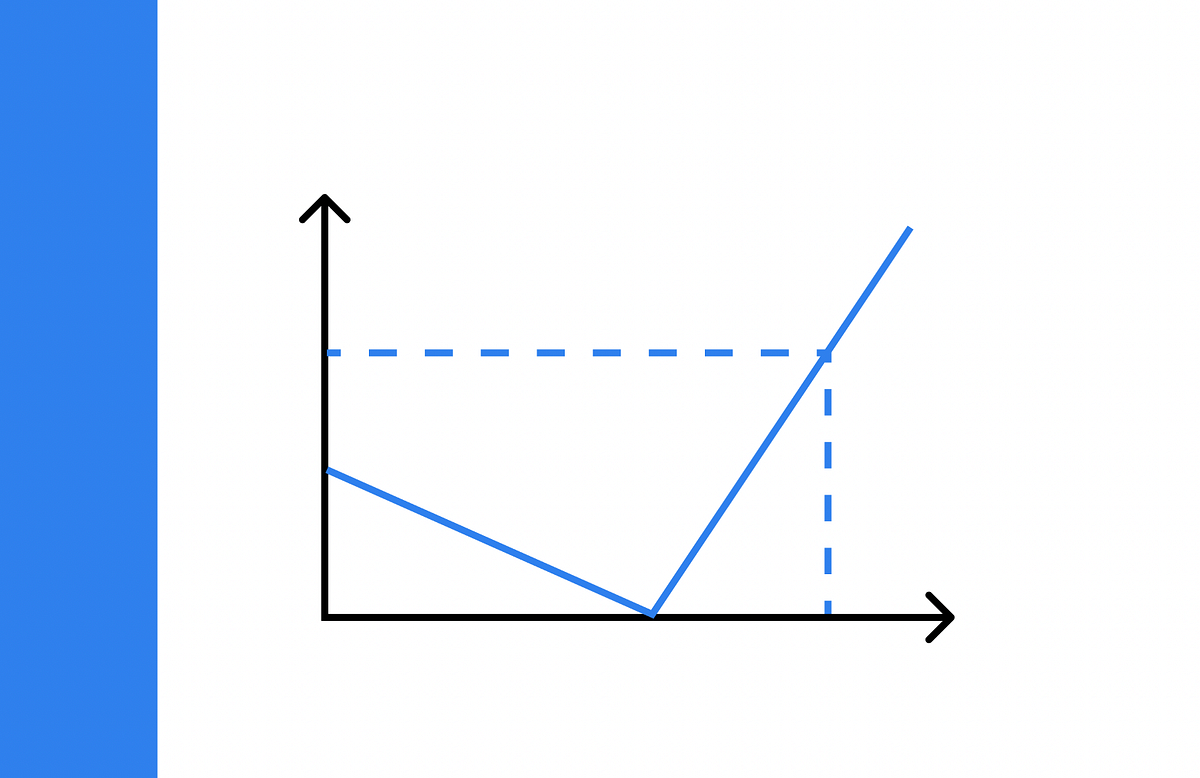
The quantified loss formula is illustrated below. α The parameter refers to the quantile that needs to be predicted.

The value of the quantile loss depends on whether the prediction is lower or higher than the true value. To better understand the reasoning behind this, consider that our objective is to predict the 80th quantile, such that α = 0.8 is plugged into Eqs. As a result, the formula looks like this:

Basically, in such a case, the quantile loss penalizes underestimated forecasts by 4 times more than overestimated ones. This way the model will be more significant for lower prediction errors and predict higher values ​​more often. As a result, on average the fitted model will overestimate the outcome in about 80% of the cases and underestimate it in 20%.

Now suppose that two predictions are received for the same target. The target value is 40, while the predictions are 30 and 50. Let us calculate the quantum loss in both the cases. Despite the fact that the absolute error of 10 is the same in both cases, the loss value is different:

• For 30, the loss value is L = 0.8 * 10 = 8
• For 50, the loss value is L = 0.2 * 10 = 2,

This loss function is shown in the diagram below which shows the loss values ​​for various parameters α When the actual value is 40.

Conversely, if the value of α 0.2, then over-estimated predictions would be penalized 4 times more than under-estimated.

The problem of predicting quantiles of a certain variable is called quantile regression,

Let us create a synthetic dataset with 10 000 samples where the ratings of players in a video game will be predicted based on the number of hours played.

Let’s split the data on train and test in the ratio 80:20:

For comparison, let’s build 3 regression models with different α Values: 0.2, 0.5 and 0.8. Each regression model will be built by LightGBM – a library with an efficient implementation of gradient boosting.

Based on information from the official documentation, LightGBM allows solving quantitative regression problems by specifying Objective as parameter ‘quantile’ and passing the corresponding value of Alpha,

After training the 3 models, they can be used to obtain predictions (line 6).

Let us visualize the predictions through the below code snippet:

From the above scatter plot, it is clear that with more values ​​of α, the models produce more predictable results. Additionally, let us compare the predictions of each model against all target values.

This leads to the following output:

The pattern is clearly seen from the output: for any αEstimated values ​​are approximately greater than actual values α * 100% of matters. Therefore, we can empirically conclude that our prediction model works correctly.

The prediction errors of the quantile regression model are approximately negative in α * 100% are positive in matters and (1- α)* 100% of cases.

We’ve explored the quantile loss – a flexible loss function that can be incorporated into any regression model to predict a certain variable’s quantile. Based on the example of LightGBM, we saw how to adjust the model so it solves the quantile regression problem. In fact, many other popular machine learning libraries allow quantile loss to be set as a loss function.

The code used in this article is available at:

All images by the author unless otherwise noted.